Meltwater recently released a new product feature called Signals, which helps our customers to identify business-critical events. One of the technical systems powering these Signals is a custom-built Knowledge Graph.
In this post we explain how we created a record linking service that utilizes machine learning and big data tactics to cluster millions of related entities from various sources with high accuracy for our Knowledge Graph.
As we are going pretty deep into the material, this post is intended for software engineers with an interest in data science or data engineering.
What is Record Linking?
Record linking, also known as entity resolution, is a method which clusters database records / knowledge base entries such that each cluster corresponds to a single distinct real-world entity (e.g., a business, a person). It is a crucial step in data cleaning and data integration.
As an example, consider the following 6 business listings, each represented by 4 attributes (name, street address, city and phone number) from various sources:

Table 1: Record linking example with Starbucks outlets (source)
The correct clustering of these records is 3 clusters that correspond to 3 actual Starbucks outlets (indicated by colors above): records \({r1, r2, r3}\) forming the first cluster, \({r4}\) the second and \({r5, r6}\) the third.
The Challenges of Record Linking
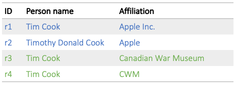
The most common challenge is that attribute values of related records will often not match literally, as in records \(r1\) and \(r2\) in the example below, both being about Apple’s CEO:

Table 2: Persons record linking example
Having identical values for some attributes however does not necessarily mean assignment to identical clusters (person names for records \(r1\) and \(r3\) above). On the other hand, some attribute values might not match at all for records that still need to go into the same cluster (affiliation attribute for records \(r3\), \(r4\) above).
We sometimes also need to work with records that are incomplete (missing attribute values), as in the Starbucks example above for record \(r6\).
Last but not least, the millions of records in our input result in big data constraints. Our solution has to be:
- Scalable. For example, comparing every record with every other one in order to find clusters would require \(n*(n-1)/2 = O(n^2)\) comparisons for \(n\) records, which would be unacceptable runtime complexity (if processing 100K records would take 60 seconds, processing 1M would take 6,000 seconds)
- Parallelizable, so we can further reduce processing time by executing computation in parallel on a cluster of physical hardware.
Record Linking for the Knowledge Graph
The Knowledge Graph (KG) is a graph-structured database where vertices represent business entities like organizations, key persons, industries, stock indices, addresses etc., while edges represent relationships like affiliations, subsidiaries, industry associations or events like mergers and acquisitions etc. The core of the KG is fused from 10+ different knowledge sources that include structured databases like Wikidata or Crunchbase. That core is continuously enriched by linking entities and adding relationships identified by NLP algorithms within editorial and social content, harvested by Meltwater daily by the millions.
Record linking is a crucial step in merging data from the different sources contributing to the KG. To take an example, here is the Wikidata entry and Crunchbase entry for Meltwater Group. We want to have a single graph vertex representing Meltwater Group, combined from the knowledge in the source records, rather than separate graph vertices from each, which would be duplicates and hence an error .
The Record Linking Pipeline
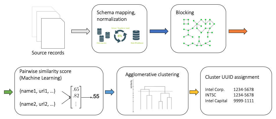
The record linking workflow is integrated into the pipeline that extracts, transforms and fuses data forming the KG, and consists of the following steps:
- All incoming source data records are validated and mapped onto a common data schema which we call the KG Ontology, so we’re able to refer to all attributes using a “common language” no matter where the data came from.
- To avoid having to execute \(O(n^2)\) pairwise comparisons, we first partition the data into blocks of records that share blocking keys. These are hash-like values calculated with easy-to-compute functions, chosen to minimize the probability that records that need to belong to the same cluster are assigned to different blocks.
- A supervised machine learning classifier then compares all records within the same blocks and assigns a probability score between 0.0 (unidentical) and 1.0 (identical) to each record pair. The classifier learns the “weight” each attribute plays in the process of deciding whether two records are identical.
- Hierarchical agglomerative clustering is then applied to the similarity matrix calculated by the classifier for each block. It is an iterative process that merges the 2 most similar records/clusters until a predetermined inter-cluster similarity threshold level is reached. Records not similar enough to other records/clusters are assigned their own singleton clusters.
- Finally, source record clusters are fused by our TruthFinder algorithm implementation into final KG vertices. This process is able to combine conflicting attribute values from various sources with the help of a learning process.
We implemented record linking in Python on top of Apache Spark to enable parallel processing, allowing us to run jobs in a distributed manner on AWS Elastic Mapreduce (EMR) clusters. The machine learning code is based on Spark’s MLlib.
In the next section, we’ll describe the details of the blocking and machine learning steps for the two most important/challenging KG types: organizations and persons.

Figure 1: The record linking workflow
Models: First Version
Organizations
To train the similarity model for the linking of organization records, we hand-picked 18 company records from 4 data sources that map to 7 manually identified clusters. We created 36 positive training examples (pairs of records that are “the same”) by taking all possible record pair combinations from within the clusters. 135 negative training examples (pairs of records “not the same”) were formed from all the 2-combinations of records across different clusters.
The training examples (positive or negative record pairs) have to be converted to feature vectors (n-tuples of floats) to be interpreted by the ML algorithm (Logistic Regression). Feature values are calculated for every record pair by
- Applying custom normalization functions to the attribute values
- Applying similarity (distance) functions to the pairs of normalized attribute values.
For organizations, we used 2 attributes, OrganizationName and HomepageURL. Normalization of OrganizationNames consisted of:
- Removing prefixes like “The”, or tokens like the possessive “‘s”
- Removing company suffixes like “Inc.”, “Corp.”, “Group” etc.
- Slugification to normalize capitalization, accents and punctuation variations.
To compare normalized OrganizationName values, we used minimum Jaro-Winkler distance, an edit distance string similarity metric that gives more favorable ratings to strings that match from the beginning for a set prefix length. By “minimum” we mean that in case there are more than one name variants to compare on either side, we return the minimum distance calculated between all possible pairs.
We normalized HomepageURLs by removing everything but the subdomain, domain, the top-level domain and the path parts of the URL. As our similarity function we chose the minimum normalized Levenshtein distance (range constrained to [0, 1]) in this case.
The following table illustrates normalization and similarity feature generation for a pair of company records represented by their OrganizationName and HomepageURL attributes:

Table 3: Organization records with normalized attributes and similarity features
During training, the Logistic Regression model learns \(n=2\) parameters, which define an optimal n-dimensional shape separating the positive and negative training examples in the n-dimensional feature space. These learned parameter values will then be used as weights for the respective feature values when we apply the model to get similarity predictions during record linking.
For the blocking of organization records, we used the domain part of their HomepageURL attributes as blocking keys (eg. would be “acme” for both URLs in the above example). This simple approach allowed a good first estimation. In subsequent experiments, we had to create a whitelist of website “hosting” domains like wordpress.com, sites.google.com, facebook.com etc. For such URLs, we kept the path part in the blocking key, eg. “facebook/acme”. This helped to rectify Spark worker out-of-memory failures by avoiding the formation of unnecessarily large blocks (eg. all the organizations having a webpage on wordpress.com would otherwise end up in the same block).
Persons
To train the first version of the similarity model for persons, we created training examples by leveraging implicit links between 2 of our data sources that contained person records. Our Wikidata source has references to Wikipedia URLs for a number of its entries, which can be automatically converted to DBpedia URLs, which uniquely identify entries in that other source.
We generated 5,000 positive training pairs by random sampling the automatically linked Wikidata and DBpedia person record pairs. To diversify the training set, we created two types of negative training examples: 5,000 “near negative” pairs, where the normalized name of the 1st record was equal to or similar in the other record, but the pair was not linked, and another 5,000 “far negative” randomly chosen, unlinked, unrelated record pairs.
We used these normalization methods for PersonName, BirthDate and Gender attributes:
- PersonName normalization #1: slugification to collapse punctuation, accent and capitalization differences, eg. HANS André Jensen → hans-andre-jensen
- PersonName normalization #2: parse the name to separate the given name and family name parts from others (middle names, titles etc.), then use a dictionary to convert given name to formal version and return this rejoined with the family name only, eg. Timothy Donald Cook, Tim Cook → Timothy Cook
- Birthdates: identify and normalize year, month and day parts (if available)
- Gender: map value to either of “female”, “male” or “other”
Through experiments we found that these 8 features yielded the best evaluation metrics for the classifier:
- Binary feature from exact matching of PersonName normalization #1 and #2: returns “1” if the two records share at least one normalized name, “0” otherwise
- 3 binary features from normalized BirthDates: exact matching of Y & M & D parts, or just Y & M parts or just the Y part
- Binary feature from exact match of normalized Gender values
- 2 special binary features that encode whether the value is missing on either side for BirthDate and Gender. This improves classification accuracy by forcing the model to distinguish between non-missing unequal values and inequality because of a missing value.
For the blocking of person records, we used slugified values from PersonName normalization #2 as blocking keys, for example:
- Jim Hackett, James Hackett → james-hackett
- Robert Iger, BOB IGER → robert-iger
- Donald M. Casey Jr., Donald Casey → donald-casey
Stay Tuned …
Curious to see how these models performed and how we could incorporate human feedback to improve them? We will publish all of this in a part 2 of this blog post in the coming weeks.
Update:
We published Improving Record Linking for our Knowledge Graph. There we share how we improved our models based on user feedback.
