Meltwater has been providing sentiment analysis powered by machine-learning for more than 10 years. In 2009 we deployed our first models for English and German. Today, we support in-house models for 16 languages.

In this blog post we discuss how we use deep learning and feedback loops to deliver sentiment analysis at scale to more than 30 thousand customers.

What is Sentiment Analysis?

Sentiment analysis is a field within Natural Language Processing (NLP) concerned with identifying and classifying subjective opinions from text [1]. Sentiment analysis ranges from detecting emotions (e.g., anger, happiness, fear), to sarcasm and intent (e.g., complaints, feedback, opinions). In its simplest form, sentiment analysis assigns a polarity (e.g., positive, negative, neutral) to a piece of text.

Let us look at a few examples:

Acme

is by far the worst company I have ever dealt with.

This sentence clearly expresses a negative opinion. The sentiment is carried by “worst company” (the sentiment phrase) and is directed at “Acme” (the sentiment target).

Tomorrow, Acme and NewCo will release their latest revenue data

In this case, we only have a factual statement about “Acme” and “NewCo”. Its polarity is neutral.

NewCo

became the first retirement plan to amass $1 trillion in assets on its platform, bolstered by record sales numbers over the past year and a surging stock market.

This time, we have phrases like “bolstered”, “record sales”, referring to “NewCo” in a positive context.

Meltwater has been providing sentiment analysis powered by machine-learning for more than 10 years. The first models were deployed in 2009 for English and German; we now have in-house models for 16 languages: Arabic, Chinese, Danish, Dutch, Finnish, French, Hindi, Italian, Japanese, Korean, Norwegian, Portuguese, Spanish, and Swedish. Most of our customers analyze sentiment trends via our Media Monitoring dashboards (Figure 1) or via reports. Larger clients, access our data via the Fairhair.ai data platform as a stream of enriched documents.

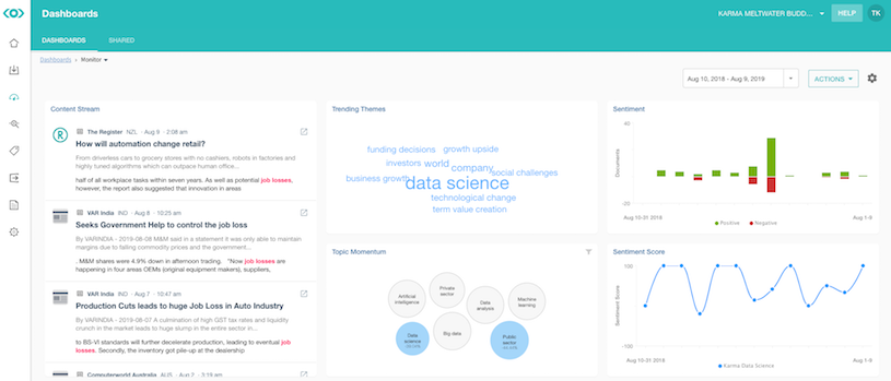
Figure 1: A Meltwater Media Intelligence dashboard.

An important feature of our offerings has always been the ability to override the sentiment values assigned by our algorithms. Overrides are indexed as different “versions” of the same document in Meltwater’s Elasticsearch cluster, providing customers with a personalized view of their sentiment when building dashboards and reports (Figure 2).

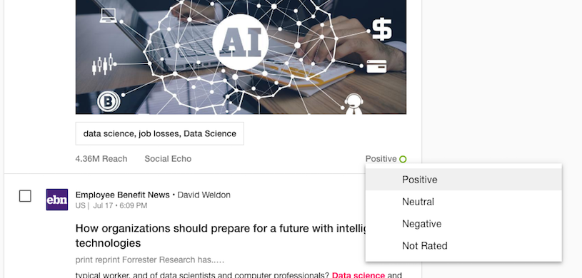
Figure 2: Sentiment override dropdown in Meltwater’s media intelligence content streams.

Every month, our customers override sentiment values on about 200,000 documents. That’s 6,500 documents every day! So why is sentiment so hard to get right?

Challenges with Getting Sentiment Right

There are certain nuances of human language that are traditionally associated with being challenging for sentiment analysis. Some notable ones are:

Handling negation:

How is your company doing? Not too bad! I am not super happy with the latest financials though…

We have three sentences here, the first is neutral, the second is positive but contains “too bad” which is usually used in negative contexts, and the third one is negative but contains “super happy”.

Sarcasm: In a sentence like

It’s raining again today… fun times!

Despite the expression “fun times”, this text is probably sarcastic and expressing a negative mood.

Comparisons:

I love the new Acme phones, they are so much better than NewCo’s.

Here expressions like “love” and “much better” carry positive sentiment, however, the sentiment is not so good for “NewCo” is it?

User-specific Bias: What would you say the sentiment of this sentence is?

Acme Police Dept

arrested today 8 people on suspicion of assault and robbery. The gang has been terrorizing the community for months.

All of the above require understanding the context in addition to the meaning of words.

A more practical problem that one has to tackle is the trade-off between accuracy and speed. Meltwater performs sentiment analysis on about 450M documents every day ranging from tweets (averaging about 30 characters in length) to news and blog posts that can reach 600-700 thousand characters in length. Each document must be processed within 20 milliseconds. We can’t afford to go much slower than that. Traditional machine learning methods such as Naïve Bayes, Logistic Regression and Support Vector Machines (SVM) are widely used for large-scale sentiment analysis because they scale well. It has now been proven that Deep Learning (DL) methods achieve better accuracy on a variety of NLP tasks, including sentiment analysis, however, they are typically slower and more expensive to train and operate [2].

The “old” Approach: Bayesian Sentiment

Until now, Meltwater has been using a multivariate naïve Bayes sentiment classifier. The classifier takes a piece of text (e.g., a document) and transforms it into a vector of features with certain values \((f_{1},\ f_{2},...,\ f_{n})\). The classifier then computes the most likely sentiment polarity \(S_{j}\), i.e. positive, negative, or neutral, given that we observed certain feature values in the text. This is usually written as a conditional probability statement: \[p(S_{j}\ |\ f_{1},\ f_{2},...,\ f_{n})\]

The most likely sentiment polarity is obtained by finding the \(S_{j}\) that maximizes the formula below. \[log(p(S_{j}) + log(p(f_{i}\ |\ S_{j}))\]

If you are interested in how the above formula is derived, click here.

Let us apply the above theory to our sentiment problem. The values of \(p(S_{j})\) are the probabilities of finding a document with a certain polarity “in nature”. These probabilities can be estimated by labelling a large corpus of documents as positive, negative, or neutral, and then computing the probability of finding a document with a given polarity in it. Ideally, we should use all of the documents ever written but that’s… impractical.

For example, if the corpus consists of the following labelled documents \[D_{1}:\text{My phone is not bad (POS)}\] \[D_{2}:\text{My phone is not great (NEG)}\] \[D_{3}:\text{My phone is good (POS)}\] \[D_{4}:\text{My phone is bad (NEG)}\] \[D_{5}:\text{My phone is Korean (NEU)}\]

Then the values of \(p(S_{j})\) are: \[p(POS) = \ 2/5 = 0.4\] \[p(NEG) = 2/5 = 0.4\] \[p(NEU) = 1/5 = 0.2\]

We use a simple Bag of Words model to derive our features. We use unigrams, bigrams, and trigrams. For example \(D_{1}\) is transformed into: \[\text{(My, phone, is, not, bad, My phone, phone is, is not, not bad, My phone is, phone is not, is not bad)}\]

The values of \(p(f_{i}\ \vert\ S_{j})\) are then the probabilities of seeing a certain feature in a document labelled as \(S_{j}\) in the corpus. We can compute their values using Kolmogorov’s definition of conditional probability \(p(f_{i}\ \vert\ S_{j}) = \frac{p(f_{i} \cap S_{j})}{p(S_{j})}\), i.e., the probability of \(f_{i}\) conditional to \(S_{j}\) is equal to the probability of \(f_{i}\) and \(S_{j}\) occurring together, divided by the probability of \(S_{j}\). For example, for the feature “bad” we have: \[p(bad\ |\ POS) = \frac{p(bad\ \cap POS)}{p(POS)} = \frac{0.2}{0.4} = 0.5\] \[p(bad\ |\ NEG) = \frac{p(bad\ \cap NEG)}{p(NEG)} = \frac{0.2}{0.4} = 0.5\] \[p(bad\ |\ NEU) = \frac{p(bad\ \cap NEU)}{p(NEU)} = \frac{0}{0.2} = 0\]

Given a document, e.g., “My tablet is good”, the classifier computes a “score” for every polarity based on the text’s features, e.g., for \(\text{POS}\) we get: \[log(\ p(POS\ |\ {my,\ tablet,\ is,\ good,\ my\ tablet,\ tablet\ is,\ is\ good,\ my\ tablet\ is,\ tablet\ is\ good)}_{})\]

which is proportional to \[log(\ p(POS)\ ) + log(\ p(my\ |\ POS)\ ) + \ ...\ + log(\ p(tablet\ is\ good\ |\ POS)\ ) = \ - 13.6949\]

We do the same for neutral and negative, resulting in the following ranking: \[log(p(POS\ |\ ...))\ = \ - 13.6949\] \[log(p(NEU\ |\ ...))\ = \ - 16.9250\] \[log(p(NEG\ |\ ...))\ = \ - 18.1709\]

The classifier then returns \(\text{POS}\) as the most likely polarity.

A Naïve Bayes classifier runs fast, since the computations required are simple sums and logarithms. However, there are limitations to what this approach can achieve in terms of accuracy, for example:

• Accurate classifications rely on representative datasets, i.e., if the training set is biased towards a certain polarity (e.g., neutral) our classifications will likely be biased as well. Accuracy also depends on having training corpora covering enough of the language we care about.
• Naïve Bayes makes strong assumptions on the independence of the features, making the underlying probabilities unreliable, even if the final ranking of polarities is correct [3,4].
• Using documents as the granularity of the training labels often leads to poor classifications when using Naïve Bayes with Bag of Words models.
• N-gram contexts are a blunt instrument. If limit ourselves to 3-grams we can’t capture correctly an expression like “not quite as bad” which is a 4-gram. However, increasing the size of the context will blow up the features space, making the classifier slower but not necessarily smarter.

Meltwater’s NLP team was tasked with improving the sentiment for all supported languages. Since training new models is a complex and expensive endeavor, the team first looked at quick ways of improving the sentiment with the technology stack we had available.

Improvement 1: Sentence-level Training and Classification

The first change we made was the way we train our Bayesian models. Instead of training and classifying at the granularity of the whole document, we are now training and classifying at sentence level. Here are some of the advantages:

• it is easier to assign a label to a single sentence (or in-context expressions) than an entire document, so we can crowdsource labels for our training sets.
• over the years, academic research produced freely-available labelled datasets for sentiment analysis evaluation. Most of these are at sentence level so we can incorporate them in our training sets.
• We can use sentence-level sentiment together with named-entity and key-phrase extraction to provide entity-level sentiment (ELS).

We then decided to aggregate the sentence-level sentiment into document-level sentiment via a stacked classifier “picking” the sentiment of meaningful sentences to produce the sentiment for the entire document (a rudimentary but effective form of attention).

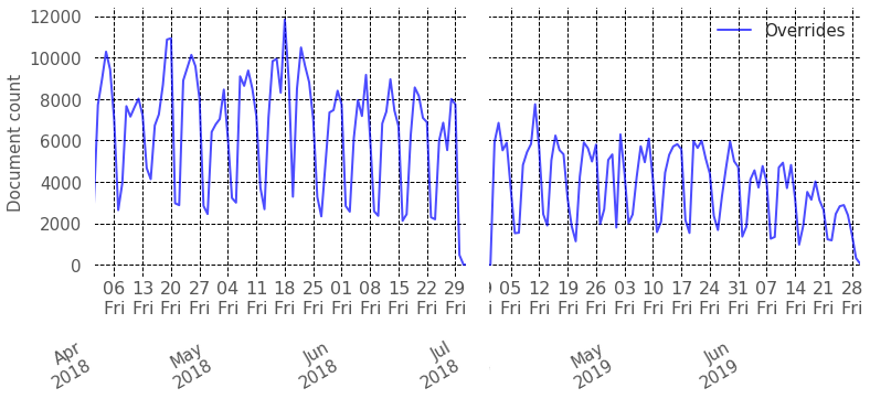
Figure 3: Overrides recorded in Q2/2018 (left) and Q2/2019 (right) - All languages.

These simple changes had a massive impact in reducing the number of overrides that our customers produce every month. In particular, overrides on news documents reduced by 58% on average across the 16 supported languages. The analysis involved around 450M news documents and 4.2M overrides produced by 7,193 customers. Figure 3 shows a comparison between overrides made Q2/2018 (document-level prediction) and Q2/2019 (sentence-level prediction + aggregation).

Improvement 2: New Deep Learning Models

In the meanwhile, the NLP team has been working on modernizing our technological stack for sentiment analysis for two key languages, i.e., English and Chinese, covering about 40% of the daily content processed by Meltwater. We experimented with a number of technologies, like Convolutional Neural Networks (CNNs), Recurrent Neural Networks (RNNs), and Long-Short Memory networks (LSTMs), with the goal of finding a good compromise between accuracy, speed, and costs.

We decided for a CNN-based solution because of the good trade-off between accuracy, speed, and running costs. CNNs are mostly used for Computer Vision but they have been shown to perform really well for NLP as well. Our solution is implemented in Python using Tensor Flow, NumPy (with MKL optimizations), GenSim, and EKPhrasis for supporting hash/cash tags, emojis, and emoticons.

Architecture: A simplified architecture is as shown in Figure 4. It consists of an embedding (input) layer, followed by a single convolution layer, then max-pooling and softmax layers [5].

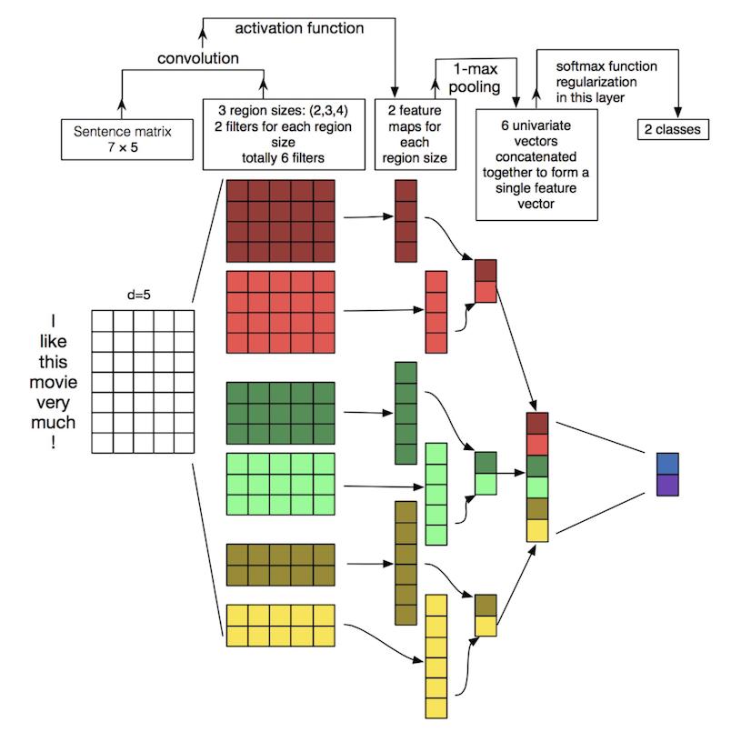
Figure 4: Simplified model architecture (Source: Zhang, Y., & Wallace, B. (2015). A Sensitivity Analysis of (and Practitioners’ Guide to) Convolutional Neural Networks for Sentence Classification)

Embedding layer: Our input is the text to be classified. As for the Bayesian case, we need to represent the text in terms of its features. We embed the text as a matrix. For example, the text “I like this movie very much!” is represented as a matrix with 7 rows, one per word. The number of columns depends on the features we want to represent. Differently from the Bayesian case, we no longer engineer the features ourselves. Instead, we now use pre-trained third-party word embeddings. Word embeddings capture semantic similarity at scale. These embeddings are publicly available and produced by neural networks trained by third-party machine learning experts. For English, we use Stanford’s GloVe) embeddings trained on 840 billion words from Common Crawl and using vectors with 300 features. We tried BERT and ElMo as well but the accuracy/cost tradeoff was still in favour of GloVe. For Chinese, we use TencentAI’s embeddings, trained on 8M phrases with vectors of 200 features. Vectors are fine-tuned via transfer learning using our own training datasets. The goal is to make sure the embeddings take into account the PR/Marketing requirements of Meltwater.

Convolution layer: At the heart of CNNs is the convolution layer, where artificial neurons are trained to extract salient features out of the embeddings. In our case, the convolution layer consists of 100 neurons for English and 50 for Chinese. The advantage, again, is that we don’t have to try and engineer features, the network will learn the ones we need. The disadvantage is that we may not be able to tell what these features are anymore. Click here if you want details about our convolution layer and here for an explanation of the black-box problem.

Max Pooling: The idea behind pooling is to capture the most important local feature in a feature map in order to reduce dimensionality, and thus speeding up the network.

SoftMax layer: The pooled vectors are concatenated into a single vector and passed to a fully connected SoftMax layer that will perform the actual classification into polarities.

Datasets: For English, apart from the GloVe embeddings, we have 23k internally labelled sentences for news, and 60k for social, including a Twitter dataset provided by SemEval-2017 Task 4. For Chinese, in addition to the TencentAI embeddings, the dataset consists of about 38k sentences from a mix of news, social, and reviews. The dataset was annotated via crowdsourcing using Amazon’s SageMaker Ground Truth. Before training, datasets are stratified and shuffle split using the 80-20 rule, i.e., we use 80% for training and 20% for validation.

Results: Already with this simple architecture, the model yields significantly better performance at sentence-level when compared to the Bayesian approach (Table 1). The gains are 7% for English social text, 18% for Chinese (combined social and news), and 26% for English news. After aggregating at document-level, we observe a further reduction in the amount of document-level overrides by 48.06% for English and 29.24% for Chinese compared to the Bayesian approach.

Table 1: Sentiment accuracy CNN vs Naïve Bayes (English and Chinese).

How accurate can sentiment analysis really be? The F~1~ score basically measures how well the model agrees with human annotators. Research tells us that human annotators only agree on the outcome in 80% of the cases. In other words, even assuming a 100% accurate model, humans would still disagree with it in 20% of the cases [6]. In practice, this means that our CNN models are doing almost as well as humans annotators in classifying single sentences.

Continuous Improvement

Until now, sentiment overrides have never been fed back to the sentiment models. The NLP team has now designed a feedback loop enabling the collection of cases where our customers disagree with the CNN classifier, so that we can improve the models over time.

Overridden documents are then sent to Fairhair.ai Studio (Figure 5) where annotators re-label them at every level, i.e., entity, sentence, section (i.e., title, ingress, body), and document.

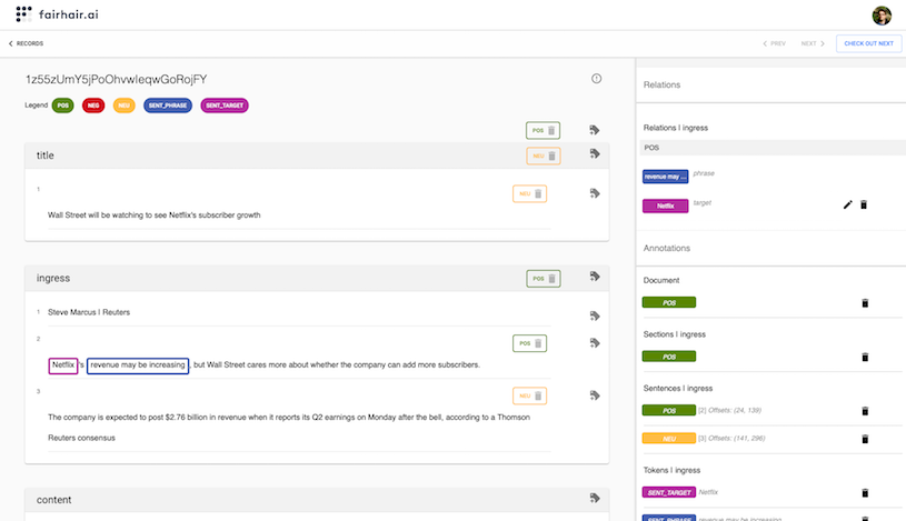
Figure 5: Fairhair.ai Studio: Meltwater’s annotation tool.

Each document is annotated multiple times by different annotators, undergoing a final review process by senior annotators to reconcile hard cases. End customers are sometimes involved in this process. When our annotation crew is not proficient in a specific language, labelling is offloaded to third-party crowdsourcing tools. Meltwater is a heavy user of Amazon’s SageMaker Ground Truth (Figure 6). When crowdsourcing is used, we increase the number of annotators required since they may not be as accurate as our internally-trained ones.

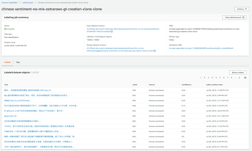
Figure 6: AWS SageMaker GT helping Meltwater labelling 2,690 Chinese documents 5 times.

After annotation is complete, the new data points are reviewed by our research scientists. The review process includes making sure that the overrides are not trying to purposely bias our model, or representing a specific customer bias requiring a specialized model. If the data is sound, it is added to the test set, i.e., we don’t want to overfit that data point by adding it to the training set. We need the model to be able to generalize the correct answer from other data points. We will collect data which is similar in nature and carries the necessary knowledge to correctly classify the overridden document. For example, if we find that the misclassification occurred in a document discussing financial products, then we will collect financial documents from our Elasticsearch cluster.

In Summary

• We changed the way we train and apply our Bayesian sentiment models for all languages, this has reduced the number of document-level overrides by an average 58% on news documents.
• We now support sentence-level and entity-level sentiment for all 16 languages. An entity for us is either a named entity, e.g., “Ford” or a key phrase, e.g., “customer service”.
• We deployed deep learning sentiment models for English and Chinese. Their sentence-level accuracy is 83% for English and 76% for Chinese. They further reduced document-level overrides on news documents by 48.06% for English and 29% for Chinese.
• The new models take into account hashtags, e.g., #love, emojis, and emoticons, including (single-line) eastern ones ( ﾟヮﾟ).
• We have a feedback loop in place to continuously improve our sentiment models.

If you have questions about this topic, please comment below or send an email to one of the authors.

About the Authors:

Stanley Jose Komban, PhD is a Senior Research Scientist at Meltwater. [pubs]

Raghavendra Prasad Narayan is a Senior Research Scientist at Meltwater.

Giorgio Orsi, PhD is a Principal Scientist and Director of Engineering (NLP) at Meltwater. [pubs]

References:

[1] Bing Liu. Sentiment Analysis: mining sentiments, opinions, and emotions. Cambridge University Press, 2015.

[2] Daniel Justus, John Brennan, Stephen Bonner, Andrew Stephen McGough. Predicting the Computational Cost of Deep Learning Models. IEEE Intl Conf. on Big Data. 2018.

[3] Irina Rish. An empirical study of the naive Bayes classifier. IJCAI Work. on Empirical Methods in AI. 2001.

[4] Alexandru Niculescu-Mizil, Rich Caruana. Predicting good probabilities with supervised learning. Intl Conference on Machine Learning. 2005.

[5] Ye Zhang, Byron Wallace. A Sensitivity Analysis of (and Practitioners’ Guide to) Convolutional Neural Networks for Sentence Classification. Intl Joint Conf. on Natural Language Processing. 2015.

[6] Kevin Roebuck. Sentiment Analysis: High-impact Strategies - What You Need to Know: Definitions, Adoptions, Impact, Benefits, Maturity, Vendors. 2012.