
We moved 1.23 TB of sentence embeddings out of our database cluster and into Amazon S3 Vectors. The migration went live in production in July 2026, cut the workload’s run cost by roughly 90%, and rollback was a config flag at every step. This post covers why the vectors existed, what pushed us to move them, how the migration worked, and a few things we learned along the way.
Background
GenAI Lens helps brands track, understand, and improve their visibility in leading AI platforms like ChatGPT, Google AI Overviews, and Anthropic Claude. Customers want plain answers: what are models saying about us, where are reputation risks showing up, how do we stack up against competitors, and which sources are shaping those answers? We get there by running prompts against the major large language models, collecting the responses, and letting customers search them semantically (“find criticism about pricing”, “where are we compared against competitor X”).
To make that search work, every LLM model response is split into sentences, and each sentence becomes a vector embedding: a list of numbers that represents what the sentence means, so similar sentences sit near each other in vector space. We use contextualized embeddings, so each sentence vector is built with the rest of the response in mind, not on its own. Those vectors power the surfaces people actually use: an agent-facing search tool, a recommendations engine, and an internal search API.
What is a vector embedding?
A vector is just a list of numbers. In this system, each sentence becomes one of those lists, usually called an embedding. The model is trained so that sentences with similar meaning get similar lists. In practice, that means you can take a user query, turn it into the same kind of list, and find stored sentences whose vectors are nearest to it. That nearest-neighbor lookup is vector search.
Dimensionality is the length of the list. Ours are 256 numbers per sentence (256-dim float32). Distance is how we score nearness; we use cosine distance, which cares about the direction of the vector more than its raw length. You do not need the linear algebra to use the rest of this post. The important idea is: meaning becomes geometry, and search becomes “find nearby points.”
Two more terms show up throughout. A model response is the full answer from an LLM: long, and usually about more than one thing. We split that response into sentences and embed each sentence on its own, so search can return the exact sentence that matched instead of the whole answer. Contextualized means each sentence embedding is built with the surrounding response in view, not as if the sentence stood alone.
Why sentences instead of one embedding per response?
Splitting each LLM response means 20-50x more vectors, which is how we got to 185 million of them. We still chose sentence-level embeddings, mostly because the product needed it. A whole-response embedding averages a long, multi-topic answer into one point, so a narrow query like “pricing criticism” barely lands. Customers also need to see the exact sentence where a model criticized them, not a link into a 1,200-word blob. Sentence-level retrieval returns that evidence directly. The same snippets feed summaries and agent tools, where a few sentences cost a lot less context than a full response. The usual downside of sentence splitting (you lose surrounding context) is exactly what contextualized embeddings fix.
The vectors first lived in our NoSQL document database, and that was fine for v1. Response metadata was already there; built-in vector search could mix tenant/date/prompt filters with nearest-neighbor ranking in one query, and we didn’t have to stand up new infrastructure to ship.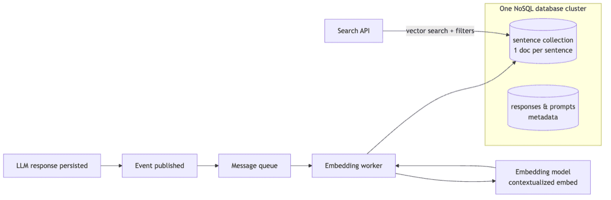
The problem
The collection grew to millions of LLM responses a day, each spawning dozens of sentence documents with a vector and text attached, and made the collection grow fast.
We tried to cut costs with an archival approach first. The latest 30 days stayed hot; everything older went to the database’s managed archive tier. Hot storage shrank, but the archive path was a federated query endpoint with no vector index, so nearest-neighbor search stopped cold at that boundary. In practice, semantic search became a 30-day feature. Even after that, the hot collection was still 1.23 TB and 185 million documents (97% of the database). That load is why the cluster had to run a sharded database, and why this workload still dominated the database cost.
That’s when the real issue became clear. We were not overpaying because search was hot and complex. We were paying it because cold data sat on a hot OLTP cluster. Sentences were never updated, everything was bucketed by day and month, and we wrote a lot more than we queried. Archival had trimmed a symptom. The storage tier was wrong, and that mismatch was the cost problem we needed to fix.
Choosing S3 Vectors
Amazon S3 Vectors (GA December 2025) puts vector indexes on S3 pricing:
- $0.06/GB-month storage
- $0.20/GB PUTs
- Pay-per-query, which means no cluster to run.
- Append-only, query-light data, that lined up.
We also priced moving the sentences into our existing hot search cluster. That option looked roughly 50% cheaper than leaving them on the OLTP cluster, but it was still hot storage for cold data, and several times the run cost we later saw on S3 Vectors.
We weren’t learning S3 Vectors from scratch either. Prompt Volume, another of our services, already used it in production for millions of monthly documents. That greenfield work had gone smoothly and left us with patterns we liked: month-partitioned index names, a fan-out reader with bounded concurrency that skips a bad month instead of failing the whole search, conservative PUT batch sizes, and one service as the only client of the store.
Limitations
topKis capped at 100 per query.- There is no count API.
- You check volumes by paginating the vector listing.
- Range filters work on numbers only.
- Strings get exact or
$inmatching.
- Strings get exact or
- Filterable metadata is capped at 2 KB per vector, total metadata around 40 KB.
- Indexing is asynchronous: a write is durable immediately but queryable shortly after.
The design
We went with one index per month, named sentences-{yyyy-MM} (cosine distance, 256-dim float32). To handle retention, we can “drop an index” instead of deleting millions of vectors. Queries only touch the months in the date range. Each index can also carry an embeddingModel tag so we have a clean seam if the model changes later.
Every vector’s key is deterministic:
{responseId}#{sentenceIndex} e.g. 665f3a...#12
This was the design choice that paid off the most. A deterministic key turns PutVectors into an idempotent upsert, so retries, redeliveries, dual-write overlap with backfill, and batch re-runs all land in the same place. Context fetch is simple too: if #12 matched, neighbors are #7 through #17 by construction. Deletes are easy for the same reason. If a response has N sentences, its vectors are always keys #0 through #N-1, so we can remove them without a separate lookup.
Filterable metadata like tenant (the customer account), day, prompt, response, and model, etc stays under the 2 KB cap. Sentence text goes in non-filterable metadata so it doesn’t show up in query scan pricing. Current and previous months keep the full text. At month 3, a lifecycle job re-puts the vectors without the text (still searchable; snippets come from the source document). At month 25, we drop the index. That replaced both the 30-day hot window and the old archive, and semantic search went from 30 days of history to 24 months.
A scheduled job creates next month’s index ahead of the boundary. We never create indexes lazily on first write; the month-boundary race that invites is not worth debugging twice.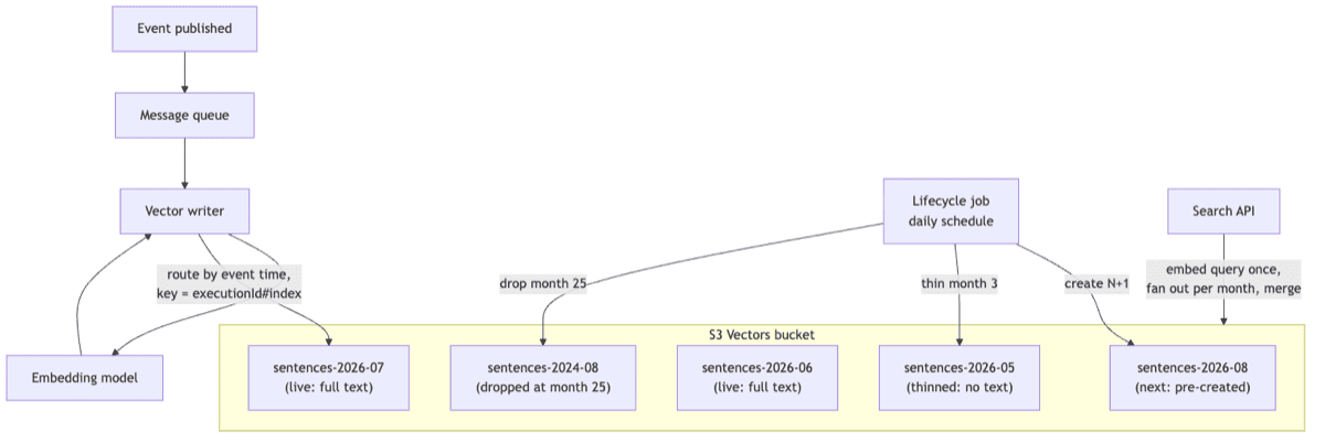
On the read path, the search API embeds the query on the server, hits each month index in the requested range in parallel, merges hits and groups them by response, then fetches neighboring keys for context snippets. S3 Vectors caps topK at 100 per query, so we cannot ask the service for more than 100 neighbors in one call. When a date range spans several month indexes, or when we need more candidate responses after grouping, we work inside that cap: over-fetch up to 100, merge across months, and if needed re-query while excluding responses we have already seen.
While backfilling history (24 months of existing sentence data into S3 Vectors), we also re-embedded everything with a newer context model. One embedding space for the whole store, and ongoing ingestion costs about 33% less per token.
The migration
We moved in small, additive steps. Every step had its own config flag so we could turn it off without undoing the rest.
- Dual write. The embedding pipeline gained a second leg writing to the monthly indexes alongside the existing database upsert. Idempotent puts meant the two writers could overlap indefinitely, so there was no deadline pressure on the soak.
- Shadow reads. The search API got a legacy v/s s3 vectors v/s shadowswitch. Shadow mode served from the legacy store while running the same query against S3 Vectors asynchronously and logging diffs: result overlap, rank correlation, latency. We cut over when the diff dashboard said parity, not before.
- Backfill. A resumable batch job walked 24 months of history, tenant by tenant, re-embedding and writing vectors. It skipped tenants without product entitlements, so we never paid to embed data nobody can query.
- Cutover. Reads first (flip the flag, watch for 48 hours, rollback is the same flag), then writes, then decommissioning after parity checks.
Problems worth knowing about
KMS and asynchronous indexing. Sentence text is customer content, so the vector bucket uses a customer-managed KMS key. S3 Vectors builds its indexes asynchronously through its own service principal (indexing.s3vectors.amazonaws.com), which means your roles having key access is not enough: the key policy itself must grant the service principal, scoped with aws:SourceAccount and aws:SourceArn, and the ARN condition must cover the bucket and its sub-resources:
{
  "Sid": "AllowS3VectorsAsyncIndexing",
  "Principal": { "Service": "indexing.s3vectors.amazonaws.com" },
  "Action": ["kms:Decrypt", "kms:GenerateDataKey*", "kms:DescribeKey"],
  "Condition": {
    "StringEquals": { "aws:SourceAccount": "<your-account>" },
    "ArnLike": {
      "aws:SourceArn": [
        "arn:aws:s3vectors:<region>:<account>:bucket/<bucket>",
        "arn:aws:s3vectors:<region>:<account>:bucket/<bucket>/*"
      ]
    }
  }
}
Two details make this easy to get wrong
Conditions like kms:CallerAccount never match service principals (the indexer isn’t calling from your account), and because indexing is asynchronous, writes keep succeeding while indexing quietly fails behind them.
Batch token limits
Embedding calls have a hard per-batch token limit, and estimating tokens from character counts under-counts dense content often enough that a high-volume pipeline will eventually submit an oversized batch. Instead of a better estimator, we wrapped the embed call in a submit-then-bisect strategy: if the provider rejects the batch or times out, split it in half and recurse, realigning result indexes across the splits. Estimation becomes a performance hint rather than a correctness requirement.
Resumable backfill
A multi-day batch will get interrupted. Getting resume right took a few tries. What worked: checkpoint the exact iteration position (tenant, month, day, last ID) and nothing derived. Document IDs don’t sort by time, and if you mix key order with time order you’ll skip or redo work without noticing. Keep a separate ledger of fully finished tenants so re-runs are safe. Lean on idempotent writes. With upserts by deterministic key, a fuzzy resume can reprocess the boundary; you might burn some embedding tokens, but you won’t lose or duplicate data.
Trade-offs
| Dimension | Verdict | Notes |
|---|---|---|
| Cost | Win | About 90% lower run cost for this workload versus the old cluster path |
| Search coverage | Win | Semantic search went from 30 days to 24 months |
| Ops burden | Win | No cluster, no sharding, no capacity planning |
| Retention | Win | Dropping an index beats deleting millions of rows |
| Query flexibility | Trade-off | topK capped at 100, numeric-only range filters; needs over-fetch and re-query patterns |
| Observability | Trade-off | No count API; verification means paginating listings; async indexing delays visibility |
| Consistency | Trade-off | Writes are queryable shortly after, not instantly; fine for us, not for everyone |
| Maturity | Watch | Young service; some behaviors (like the KMS interaction) you learn in production |
Lessons we learned
- Put the data on a tier that matches how it’s used. Append-only, time-partitioned, query-light data did not belong on a hot OLTP cluster.
- Deterministic keys and idempotent writes made the rest simpler: dual writes, retries, redrives, and every backfill resume edge case. If you only sweat one design choice, sweat this one.
- Try a new storage service on a greenfield workload before you migrate a legacy one onto it. We learned how S3 Vectors actually behaves on a new product, then moved the old workload with patterns we already trusted.
- Keep every migration step additive, with its own off switch. Approving cutover is easier when rollback is a flag flip.
- For batched provider APIs with hard limits, plan for rejection (submit, then bisect on failure) instead of betting on perfect token estimates.
- Probe a young service’s limits yourself before you commit. The query caps, missing count API, and filter rules were workable for us, but only because we designed around them up front.
Where we are now
S3 Vectors has been the live store for sentence search since July 2026, with 24 months of history searchable. Decommissioning is done too: the legacy collection and archive are gone, the database cluster is descaled, and we’re actually paying the lower bill.
And because no engineering blog post is complete without a dad joke.
Knock knock.
Who’s there?
Vector.
Vector who?
Vector who’s home in S3 now.