
For a brand, the cost of a risk is often set by how early it is noticed. A data breach, a boycott or a misleading claim can spread quickly, and the teams responsible need to see it while there is still time to respond. Reliable early detection of emerging risk, misinformation included, is therefore one of the most valuable things a media intelligence platform can offer.
Every day, Meltwater processes a continuous stream of editorial content from news outlets and blogs, and social content from social media platforms worldwide. Each document is enriched with insights such as the people and organizations it mentions, the sentiment toward each of them, and its key phrases, so customers can follow what is being said about their brands. Reputation risk classification is one of these enrichments: out of the box, it identifies reputation risks across a broad range of topics, so customers can spot emerging issues and act before they grow.
What the classifier does
The reputation risk classifier is modeled as a multi-label task, because a single article or post can be about several risks at once, such as a customer boycott, pricing complaints and product quality concerns. Behind it is a three-level taxonomy. At the top are 8 pillars, broad risk themes such as Crisis & Controversy or Brand Perception. Each pillar splits into categories (16 in total, such as Brand Scandals & Crises or Price & Value), and each category contains specific sub-categories (38 in total, such as Boycotts, Pricing Criticism or Quality Concerns & Defects). The classifier predicts at the sub-category level, so one document’s labels can span several pillars, and the higher levels let us summarize results by broader theme, as we do by pillar in the results below.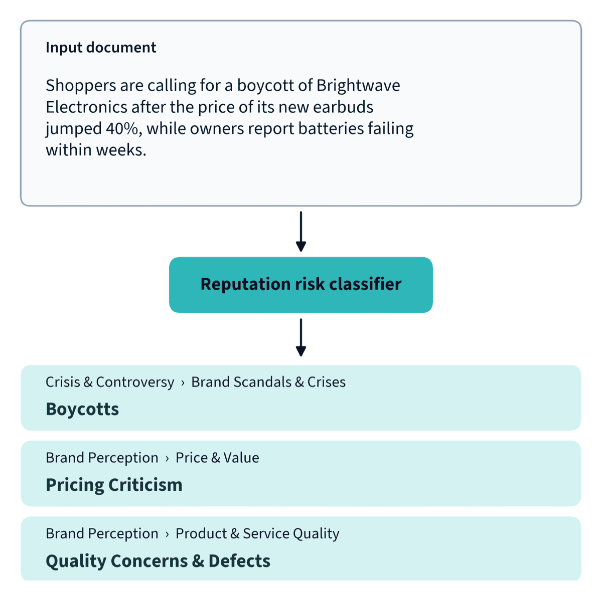
v1: our first model
Before v1, each risk label was detected by its own Boolean query. Instead of maintaining a separate query for every label, we trained a model to learn the labels from examples.
We started from a pretrained language model that turns text into embeddings (BAAI/bge-base-en-v1.5) and adapted it using contrastive learning, a technique that teaches the model to place documents with similar risks close together and unrelated ones far apart. A classification layer on top then assigns the labels. This works well with a few examples, which is what we had: roughly 100 per label, or about 2.6k training documents for the editorial model and 3.0k for the social one.
Throughout this post, we judge the classifier on two standard metrics. Precision asks: when the model flags a risk, how often is it right? Recall asks: of all the documents that really are about a risk, how many does it catch?
Raw scores alone weren’t precise enough, so we tuned a separate decision threshold for each label, deliberately favoring precision over recall.
| Precision | Recall | |
|---|---|---|
| v1 editorial | 0.824 | 0.553 |
| v1 social | 0.827 | 0.522 |
Scores throughout this post are averaged across all 38 sub-categories, so every label counts equally. These use the re-annotated test set described in the results section, so they differ slightly from those published at v1’s release.
What v1 taught us
When v1 flagged a risk, it was right about four times out of five. But it found only about half of the risks that were actually there, so a lot slipped through. Tuning thresholds for precision came at the cost of recall, and our hypothesis was that the small training set made it hard to achieve both.
The misses weren’t spread evenly. “Governance” and “Brand Perception” pillars fared worst. On the social documents, the model caught only about 1 in 5 posts about governance issues and fewer than 1 in 4 about brand perception. One possible reason is that risks like these depend more on tone and context than on concrete events, so a hundred examples may not capture the many ways people write about them.
v1 gave us a foundation to build on. To improve it, we set out to test whether more labeled data, better labels, and a stronger model could close the gap.
v2: what changed
v2 changed three things: the documents we train on, the labels we train with, and the model itself.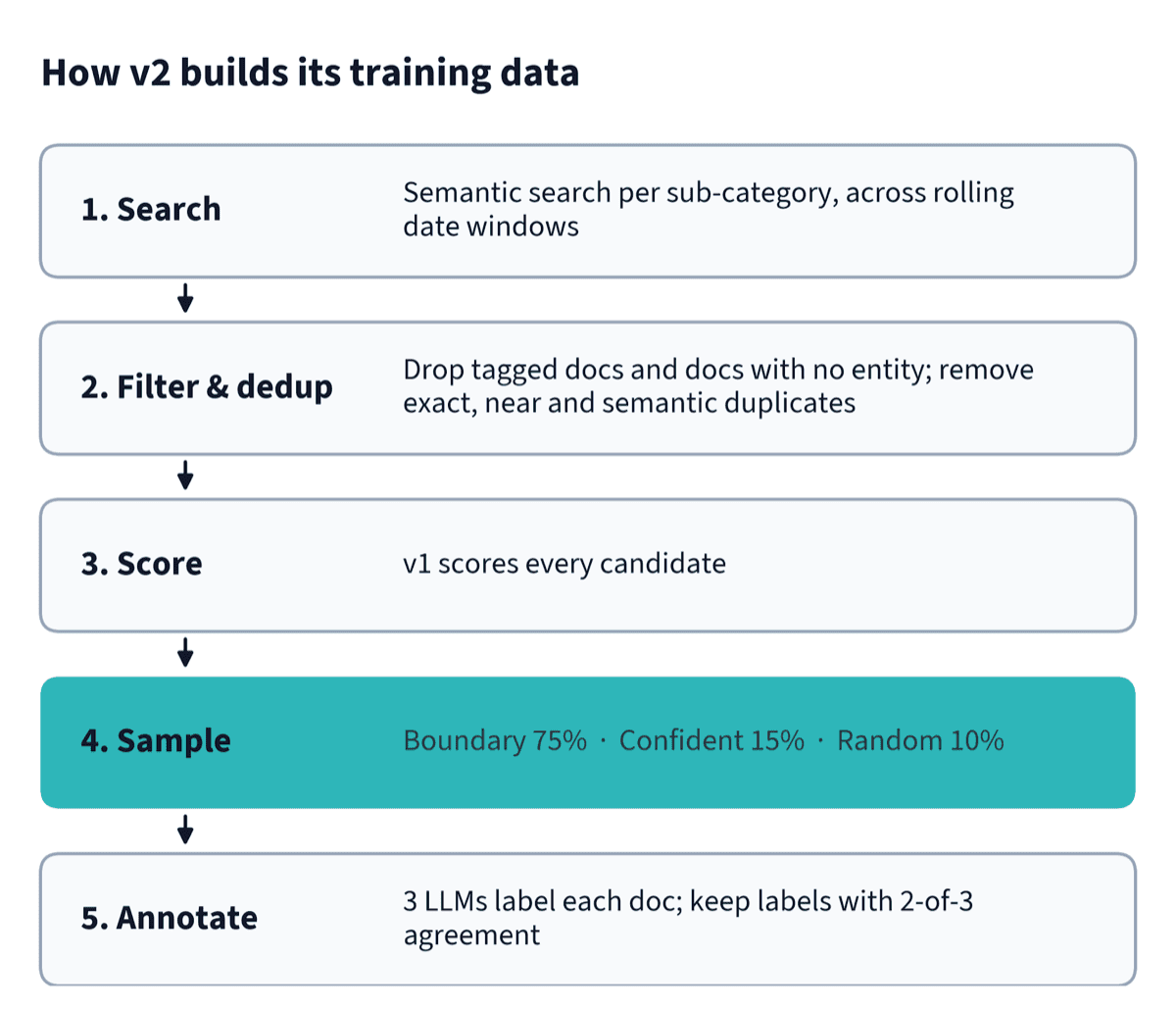
1. Better-chosen training data
For v2 we went looking for far more training data. For every sub-category, we ran a semantic search over Meltwater’s editorial and social content, using the sub-category’s name and description as the query, so documents were matched by meaning, not just by exact keywords. We repeated each search across rolling date windows spanning a full year of content, and ran it separately for editorial and social. (v1 also ran one search per label, but at a much smaller scale.) We deliberately searched beyond the subset of documents the classifier runs on in production, to capture documents that could genuinely be about reputation risk but that v1 had never scored.
From there, we excluded documents that already carried a reputation risk label, so that the pool would focus on what v1 had missed, and dropped any that mentioned no person, product or organization, since reputation risk is always tied to a specific entity. Finally, we removed exact, near and semantic duplicates.
We then had to choose which documents to label. We scored the whole pool with v1, the production model, and concentrated on the documents it found hardest to call:
- Most of the sample comes from right around the model’s decision boundary. These are the documents where the model is least certain, and where a new model has the most to learn.
- A smaller slice of confident positives keeps the clear cases in view.
- A small random slice keeps the sample anchored to what the wider pool looks like.
Because a confident prediction can still be wrong, the confident and random slices make sure the model also learns from documents beyond the boundary band. We also sampled by percentile rank rather than raw score, so every label gets a boundary band of similar size even when its scores are skewed.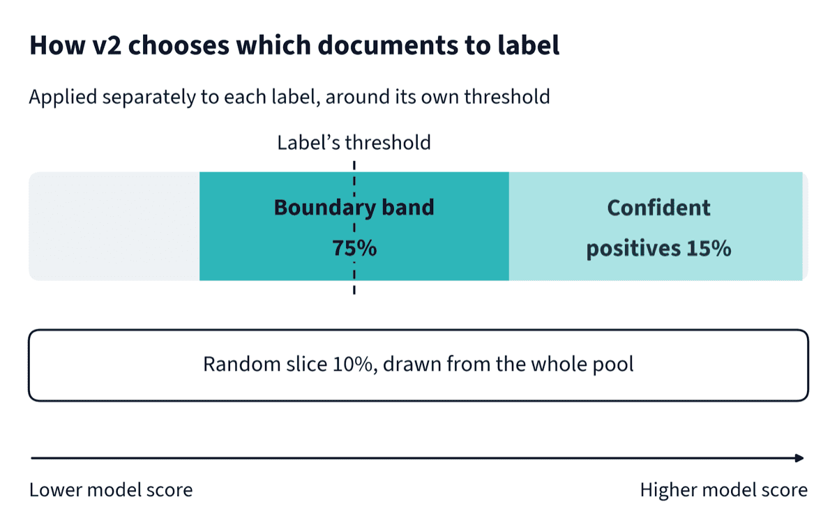
2. More precise labels
We kept v1’s annotation setup: three independent LLM providers label each document, and a label is kept only when at least two agree. What we changed was the prompt, which we found was over-labeling, assigning labels too readily. The v2 instructions tell the LLMs to assign a label only when the document is actually about that reputation risk. We also moved to newer versions of these LLMs, and tests on sample documents showed that they produced higher-quality annotations.
3. A different model
v2 fine-tunes gte-modernbert-base directly as a 38-label classifier. v1’s encoder, bge-base, is built on the original BERT architecture, which reads at most 512 tokens. gte-modernbert-base is built on ModernBERT, a modernized take on BERT that was trained on much more recent data and designed to process long inputs efficiently. That let us give editorial articles twice the context, 1,024 tokens, while social posts stay at 512. We also dropped contrastive learning, which is built for small datasets and no longer fits when training on about 90k documents per source.
Thresholds got simpler too. v1 needed a tuned cutoff for each label to reach its precision, while v2 uses the same default cutoff of 0.5 for every label and still reaches higher precision.
Results
We compared v2 with v1, the model currently in production, on the same test set. That set was built during v1, so v2’s sampling had no influence on it. It was also re-annotated with the v2 prompt and models, so both models are scored against the same labels:
| v1 → v2 | Precision | Recall |
|---|---|---|
| Editorial | 0.824 → 0.886 | 0.553 → 0.820 |
| Social | 0.827 → 0.857 | 0.522 → 0.836 |
Recall rose by roughly 0.3 on both sources, while precision rose as well.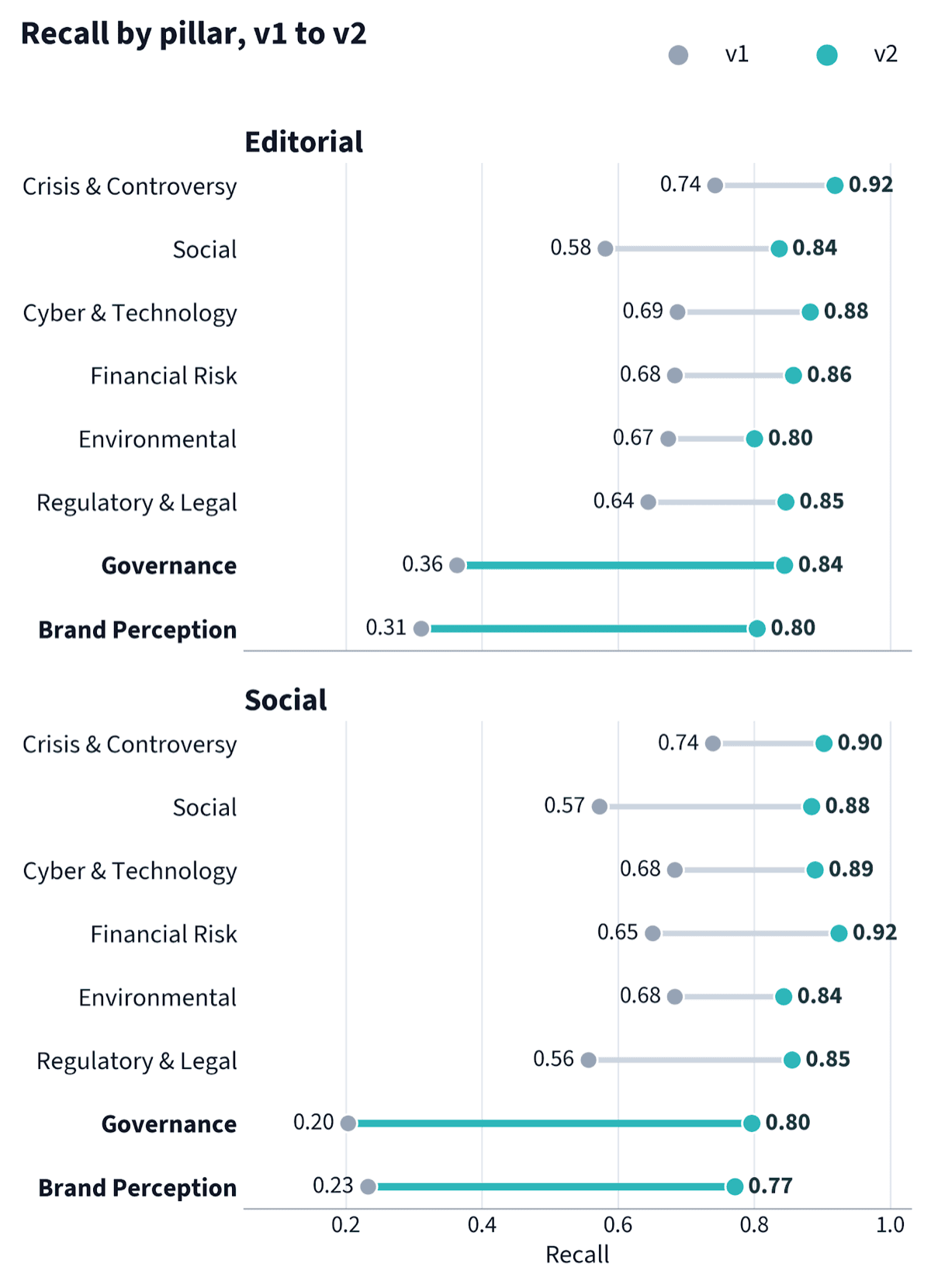
Recall improved in every pillar, and the biggest gains came where v1 had struggled most. On social posts, v1 caught about 1 in 5 in the Governance pillar; v2 catches about 4 in 5. Precision tells a steadier story. It rose or held in most pillars, with Governance the one clear exception: it gave back some precision in exchange for the largest gain in recall.
The gains came with one trade-off: on average, v2 takes slightly more than twice as long as v1 to process each document. That is still well within the time we allow for processing, so customers saw no difference, and running costs stayed the same, since v2 runs on the same computing resources as v1.
How much did the new model contribute?
To isolate the model, we trained the old bge-base encoder on the same v2 data and compared it with v2. Because both learned from identical data, any difference between them comes from the model.
| Same v2 training data | Editorial precision | Editorial recall | Social precision | Social recall |
|---|---|---|---|---|
| Old encoder (bge-base) | 0.857 | 0.732 | 0.862 | 0.782 |
| New encoder (gte-modernbert, v2) | 0.886 | 0.820 | 0.857 | 0.836 |
The new encoder catches more risks on both sources and is slightly more precise on editorial. But the model isn’t the main story: trained on the v2 data, even the old encoder already catches far more risks than v1 did. Most of the improvement from v1 to v2 came from the changes other than the encoder.
Limitations
Only the model’s contribution is isolated. Going from v1 to v2 also changed the training data, the labels and the training setup, all at once, so we can’t attribute the rest of the gain to any one of them.
Looking ahead
For customers, the difference is easy to state: v2 catches far more of the risks that matter, from governance lapses to shifts in brand perception. Next, we’re bringing the same approach to multilingual models. And because each model now helps choose the training data for the next, v2 will select the data for v3, so the work that took us from v1 to v2 is also where v3 begins.