

This is part 3 in our series on how we upgraded our Elasticsearch cluster without any downtime and with minimal user impact.
As part of the Elasticsearch Upgrade project, we needed to investigate the search performance improvements between the old and the new versions. Running an older version of Elasticsearch has presented many performance issues over the years and we hoped that upgrading to a more recent version would help.
This blog post will describe how we tested the search performance of our new Elasticsearch cluster and the different optimizations we used to improve it. Specifically, we will focus on how we solved the major bottleneck for our use case: wildcards.
Searches at Meltwater
To better understand this blog post we first need to understand how customers search on our platform. The most common way to search is to write a boolean query, for example:
Meltwater AND ((blog NEAR post) OR “search perfor*”)
The booleans are then converted into Elasticsearch queries which are executed in the cluster. Our boolean language includes lots of different query types, the most commonly used are terms, phrases, nears, range searches, and wildcards.
We categorize the wildcards into these 5 categories:
- Leading wildcards: *foo or ?oo
- Trailing wildcards: bar* or ba?
- Double-ended wildcards: *bar*
- Middle wildcards (single or multiple): b?ar*t*
- Wildcards within phrases: “foo* b*a?”
- This is a custom Meltwater feature similar to the match phrase prefix query, but with support for wildcard anywhere in the phrase
Typically, the boolean queries that our customers create are huge! We allow searches to include up to 60.000 terms and 30.000 wildcards. The boolean may also be as long as 750.000 characters. Allowing our customers to craft these massive queries is one of Meltwater’s strengths in our market, but it does create challenges for our team and Meltwater engineering as a whole.
To support these huge queries in the old cluster we’ve implemented many performance optimizations in our old forked Elasticsearch version. If you are curious to read more about the optimizations we implemented you can look at one of our older blog posts.
Maintaining custom modifications of Elasticsearch comes at a cost. It makes upgrades harder and takes time and effort to maintain. For the new cluster, we wanted to see if we could achieve the same functionality and performance by using some clever combinations of existing features from vanilla Elasticsearch.
Baseline search performance of the new Elasticsearch version
We started with a consciously simple and naive approach to our performance testing. We got the new cluster to a point where the search results passed our compatibility tests and it could handle all our live indexing. As soon as we had that we could start to compare the performance of searches.
For the old version, we already had a decently sized cluster in our staging environment that we could do comparisons against. To make the comparisons as fair as possible we made sure we used the same instance types and the same amount of data nodes in both clusters.
We then replayed production searches to both clusters and compared how long it took for requests to complete. Initially, our old optimized cluster was a lot faster than the new one, especially for all the wildcard queries. Some of our queries also triggered huge heap spikes in the new cluster, causing nodes to stop responding to pings and consequently leave the cluster.
Getting to the bottom of these problems took us several months of focused effort. In the following sections, we will describe some of the optimizations we made that had a major impact on the performance of the new cluster.
Wildcard query execution
To fully understand the rest of this blog post we first need to say a few words on how Lucene (the underlying search library that Elasticsearch uses) indexes documents and then executes wildcard queries on them.
Let’s say we want to index the following document:
{
  "text": "wildcards wont win"
}
As the document is being indexed, all the terms of the text field are also stored in a term dictionary. The term dictionary is essentially a set of all the unique terms in the field across an index. For example, if we only have our example document indexed we would have the following term dictionary:
[
  "wildcards",
  "wont",
  "win"
]
When you search on the text field using a wildcard query, Elasticsearch rewrites the wildcard into the matching terms of the wildcard. This is done by finding all the terms in the term dictionary that the wildcard matches. From the matching terms, a new Lucene boolean query is created. Note: This refers to Lucene’s BooleanQuery and not our Meltwater Boolean language mentioned previously. So, if you search for wi* (and we only have the above document in our index) then Elasticsearch will rewrite the wildcard into this Lucene boolean:
(wildcards OR win)
The rewritten Lucene boolean is then used to find which documents match the query.
Leading wildcards
Another important thing to know about Lucene is that the term dictionary is good at finding matching terms of trailing wildcards, e.g. “elasti*”. The reason is that the term dictionary is alphabetically sorted, allowing Lucene to quickly find the first term that starts with a prefix. Then Lucene can iterate the next term until it no longer matches the wildcard.
However, for leading wildcards it’s much harder to find which terms match the wildcard. There is no index structure that supports an efficient search of terms that end with some characters, for example, “*sticsearch”. In this case, Elasticsearch has to perform a regex on every single term in the term dictionary to find which ones match the wildcard. And this is orders of magnitude slower for large indices. The Elasticsearch documentation also mentions this in the wildcard queries section:
Avoid beginning patterns with * or ?. This can increase the iterations needed to find matching terms and slow search performance.
Luckily, there is a fairly easy way to optimize for leading wildcards as well. If you index all terms in reverse you can convert the leading wildcard to a trailing by first reversing the wildcard query term and then searching in the reverse field. In modern Elasticsearch versions, you can easily set this up by creating a multi-field mapping with a subfield that uses the reverse token filter.
The downside of this optimization is that it increases the disk usage by a factor of two for each field that we add a reverse index to. In our case, we didn’t need to enable this for all the fields. Most of our wildcard queries are only targeting a small subset of the available fields, primarily the title and the body text fields. With that trade-off, we ended up only increasing our index sizes by roughly 30% overall. The performance boost we got by trading off this added disk usage for less CPU and memory used at search time paid off very well for our customer’s use cases.
Wildcard rewrite limits
While the reverse index optimization greatly improved the speed of leading wildcards we still had severe stability issues in the new cluster, where many of the data nodes died from time to time.
By using a tool called Blunders.io, we could identify that most of the heap was allocated in a class called SpanBooleanQueryRewriteWithMaxClause. This code is responsible for rewriting wildcards in span nears, which are used for our implementation of the Wildcards within phrases feature that we support in Meltwater.
The typical pattern we observed was major heap spikes on data nodes which caused them to go out of memory. After they went out of memory the Elasticsearch process died and the master subsequently kicked them out of the cluster. An example of this can be seen in Figure 2.
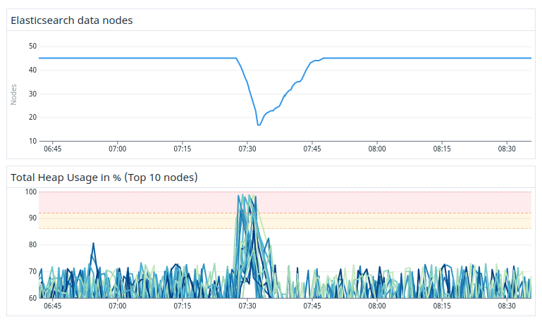
Figure 2. About 60% of all data nodes got out of memory and left the cluster.
These incidents were caused by a combination of two things; we had raised the setting indices.query.bool.max_clause_count, while at the same time a search that contained a massive amount of wildcards within phrases was executed. When those wildcards were rewritten Elasticsearch kept all the rewritten terms (the long OR chains) in memory when executing the request. And when the long list of terms was too large to fit in the heap then some Elasticsearch nodes ran out of memory and crashed.
The limit that we changed controls how large each Lucene boolean can be. When Elasticsearch rewrites wildcards it aborts the search if the limit is exceeded to prevent the memory from blowing up. In the old cluster, there was no such limit, which was a common root cause for some of the problems explained in the first post in this series.
In the old cluster, we addressed the risk of memory issues by doing changes to Elasticsearch itself. We added domain-specific heuristics, term rewrite caches and avoided some wildcard rewrites altogether by lazy evaluation of the wildcards. All of this made it possible to handle large wildcard rewrites. Eventually, we also implemented our own term rewrite limits similar to how more modern Elasticsearch versions behave. But to not affect too many of our existing users we used a limit of 100.000 terms. This is a lot higher than the default of 1024 that Elasticsearch 7 uses and the automatically calculated total limit Elasticsearch 8 uses.
Given the limit that we had in the old cluster, many of our 800.000 saved customer queries have wildcards that rewrite to more than 1024 terms. So, in our naive approach to getting the new cluster to be compatible with the old, we had to raise the default limit from 1024 to over 100.000. But given the stability issues this caused us, it became obvious that this raised limit wouldn’t work if we ever wanted a reliable cluster.
So we embarked on a quest to find a better limit for our use case. We did a series of controlled tests, lowering and lowering the limit while continuously replaying searches in the new cluster until we no longer had any major heap issues. Eventually, we concluded that the safe limit was 2.000. Sticking to that number gave us a reasonably stable cluster, even for the worst-case scenarios, which can be seen in Figure 3. You can see that there were still heap spikes, but nodes were no longer getting out of memory.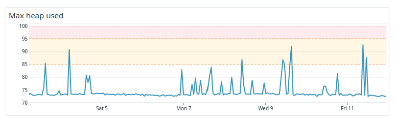
Figure 3. Improved heap usage in the cluster after limiting wildcard rewrites.
The problem with setting the limit to 2.000 however, was that it caused our new cluster to reject around 15% of all our customers’ searches, which for us meant over 100.000 in absolute numbers. It would have been an enormous task for our support organization to go through them all, change them and then verify that they still worked as intended.
We considered re-implementing the internal changes we had done in the old cluster to optimize wildcards in nears, but that would have likely delayed the upgrade by months and also again, made it a lot harder to upgrade to future Elasticsearch versions. Luckily, we instead found another way to solve this problem, namely using index prefixes.
Index prefixes
Index prefixes is a feature in Elasticsearch that basically rewrites trailing wildcards at index time. This feature index all the possible prefixes of a term in a separate subfield called _index_prefix.
For example, if you index a document with the term Monkey the _index_prefix field will then contain the terms M, Mo, Mon, Monk, Monke, Monkey. Using this index it is possible to convert a trailing wildcard query (e.g. Monk*) into a normal term query (Monk) against the _index_prefix field, without any wildcard rewriting at all. So essentially every trailing wildcard is then treated just like a regular term query, which is a huge performance gain. Note that you also need to use a prefix query for this to work correctly, but that logic was handled by our middle-layer service.
By using index prefixes the heap usage on the data nodes got a lot better, see Figure 4. In terms of stability, this is truly amazing and something we’ve hardly ever seen in the old cluster despite all optimizations and custom code.
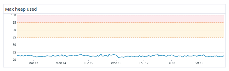
Figure 4. Heap usage after enabling index prefixes.
The downside of using this is something you might’ve guessed already, Index prefixes use a lot of disk. To avoid exploding the disk usage in the cluster we only added Index prefixes to a few selected fields that are frequently searched for with wildcards. But even then our total disk usage grew by about 60%.
Final outcomes
It might sound counterintuitive, but despite all the growth in disk usage, index prefixes made the new cluster a lot cheaper than the old one. Because of all the heap issues that wildcards caused us in the old cluster, we had to scale that cluster based on heap to guarantee stability. As index prefixes instead gave us a stable cluster in terms of heap, we could now scale on disk. This meant that we could go from 1.100 data to just 600 equivalent ones in the new cluster, reducing the cost by around 45%.
The new cluster was also a lot faster than the old one. Elasticsearch no longer had to spend lots of time rewriting and evaluating wildcards; the median search time improved by around 25% and the 95th percentile by 33%.
Index prefixes unfortunately didn’t help us with the middle or dual-ended wildcards. Luckily enough, there were a lot fewer of those searches, few enough that we could ask for help from our fantastic support organization. They helped us change all of the bad dual-ended/middle wildcards into more optimal variants.
Going forward, we now also have built-in protection against unoptimized wildcard rewrites and we can continue sleeping throughout the night knowing that Elasticsearch will reject those queries given our 2.000 boolean max clause limit.
So using index prefixes, together with the leading wildcard optimization left us with a much cheaper, stable, and more powerful cluster, all using only official vanilla Elasticsearch!
This concludes the third part of our blog post series on how we upgraded our Elasticsearch cluster. Stay tuned for the next post that will be published sometime next week.
To keep up-to-date, please follow us on Twitter or Instagram.
Up next: Part 4 - Tokenization and normalization for high recall in all languages
Previous blog posts in this series: